I created a small demo in Hugging Face Spaces to play with the code
A couple of weeks ago I saw a very interesting post by Alexander Soare and Francisco Massa on Pytorch Blog. The authors explained that the latest version of Torchivision v0.11.0 included a new utility that allows us to access intermediate transformations of an input during the step-forward of a PyTorch module. That is, we don’t need more complex code to get the intermediate activations of a model, we can simply point to a specific layer and get its results. The article analyzes the different methods that were used to carry out this task, comparing their advantages and disadvantages. This is a remarkably clear post (as generally on the Pytorch blog) that not only explains you how this new feature works, but also provides insight into the other common methods.
So … I couldn’t resist, I really wanted to try this and see how it works! I’ve been thinking about the differences between Transformer and CNN when classifying images and was wondering if I could compare them. So I rechecked the Class Activation Map paper[1] from 2015. This is a classic job that shows how to paint activation maps from your last conv layer, conditioned on your model output label. For the case of transformers, I based my experiments on Attention Flow [2] which seems to be the standard method in the community.
This post was created with the intention of improving my knowledge on ViT, TorchVision and model’s explainability. I do not pretend to compare ResNet against ViT since they have been trained with different datasets. ViT was pre-trained on ImageNet-21k and finetuned on ImageNet whileas ResNet50 was only trained on ImageNet.
Now, let’s see how to implement both methods and visualize some results!
Class Activation Map - ResNet
A small review
In [1] authors propose a way to relate last layer activations to the input image. Conv layers apply a set of filters to the input data and they return the stacked filter responses. In this paper authors show how each of this stacked responses contribute to decide the output label. The trick is very simple, they propose to add a Global Average Pooling (GAP) layer over each of the 2D features outputted from the last convolutional layer. Thanks to this, we can figure out how much is each filter contributing to the final classification of the image. As usually an image is worth a thousand words, so have a look at the figure below extracted from the paper:
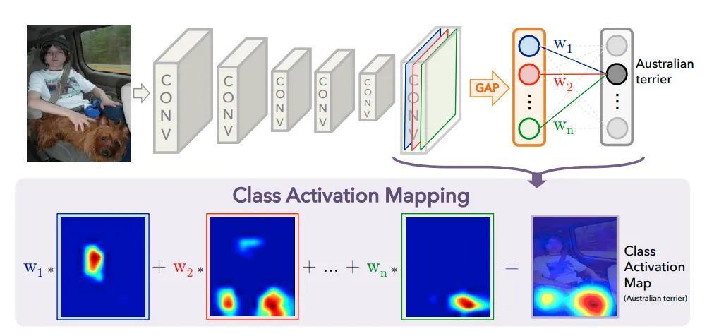
See how the GAP layer reduces each of the filter outputs to a single averaged element. Then, we will have a vector of size n_filters that will be multiplied by a linear layer which weights will be a matrix of size n_filters x n_classes. Once you know the classification output, you can “isolate” the weight vector related with that class and multiply it by the activations. In math notation this would be expressed by:
where \(k\) represents the number of filters in the last conv layer, \(w_k^c\) are the linear layer weights and \(f_k(x,y)\) represents the 2D stacked filter responses.
This paper was publised in 2015 and at that time popular architectures did not have GAP layers so they have to be finetuned with these extra layers… But we are going to use a ResNet architecture which already has a GAP layer at the end! You can check here torchvision implementation of ResNets to be sure of this.
There have been multiple works that have evolved CAM idea, you can check a few implementions of them in torch-cam repo.
Code
First of all we need to get the pretrained ResNet50 model from torchvision and put it in eval model. Then we can get extract the features we need by specifying their names. We can check all the names of the layers with get_graph_node_names function. In this case I need to extract last conv layer activation, this is layer4. One of the advantages of using the new feature extractor is that it would automatically mark the layer4 as a leaf of the computation graph, so following layers would not be computed (and that’s awesome!). Unfortunately, we also need to get the classification output of the network so we are not really getting the full power of the feature_extractor. Let’s code this:
from torchvision import models
from torchvision.models.feature_extraction import create_feature_extractor

resnet50 = models.resnet50(pretrained=True).to("cuda")
resnet50.eval()

feature_extractor = create_feature_extractor(resnet50, return_nodes=['layer4', 'fc'])
For computing the CAM we just need to apply the previous formula. First we need to get linear layer weight matrix, select the row that relates with the predicted output class and multiply it by the extracted features, then we can apply min-max normalization so that the CAM is between 0 and 1.
fc_layer_weights = resnet50.fc.weight

with torch.no_grad():
    # Extract features and remove batch dim
    output = feature_extractor(img_tensor)
    cnn_features = output["layer4"].squeeze()
    class_id = output["fc"].argmax()

    # Linear combination of class weights and cnn features
    cam = fc_layer_weights[class_id].matmul(cnn_features.flatten(1))

# Reshape back to 2D
cam = cam.reshape(cnn_features.shape[1], cnn_features.shape[2])
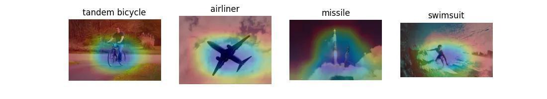
That’s all! Just a few lines, let’s see a few simple examples:
ViT Attention Map
Another brief review
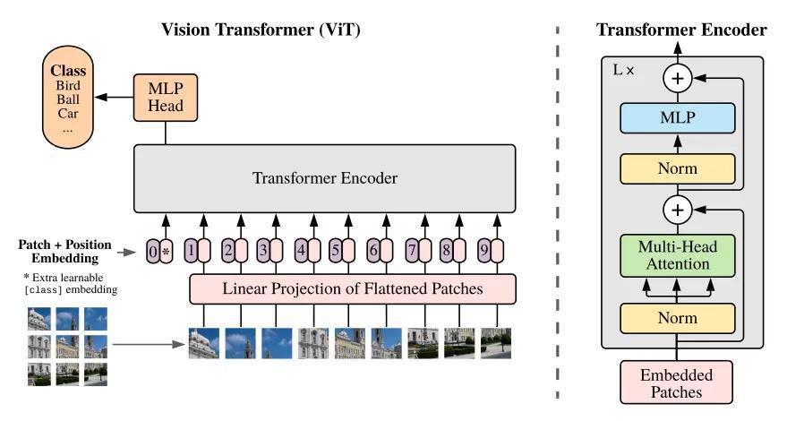
ViT paper[3] was publised at the end of 2020 and it has already become a reference in the field. There are an incredible large number of works[4] that have used it as a baseline to build new methods upon its ideas. The authors found a simple way to treat images as sequences so they can feed them to a Transformer encoder, simply divide them into fixed-size patches.
The attentions mechanism allows us to figure out what parts or patches of the image are key for the classification result. This will allow us to interpret model’s decision.
\[Attention(Q,K,V) = softmax(\frac{QK^T}{\sqrt{d_k}})V\]In the attention formula, the dot product between the query and the key represents the raw attention scores. I like to imagine this as a similarity matrix, where each position represents how “similar” the query and key embeddings are. So when both vectors are not aligned the dot product will tend to zero.
At the very first attention layer, the input vectors are the linear projections of the flattened patches:
# Pseudocode simplification from HF implementation
patch_embeddings = PatchEmbeddings(image, patch_size=16)
flat_patch_embeddings = Flatten(patch_embeddings, dim=-1)
linear_projections = Linear(patch_embeddings, out_features=embedding_size)
So it would be very easy to visualize attention weights at this very first layer because they directly relate to the image embeddings. This task becomes harder when we stack multiple Transformer layers (there are 12 layers in ViT). In [2] two different methods are proposed with the aim of easing this task, Attention Rollout and Attention Flow. We are going to use the first of them because of its simplicity.
Attention Rollout
We can model the information flow as a graph where input patches and hidden embeddings are the nodes and the edges represent the attentions from the nodes in one layer to the next layer. These edges are weighted by the attention weights which determine the amount of information that is passed from one layer to the next. Hence, if we want to compute the attention that a node at layer \(i\) receives from all previous layer nodes, we can simply multiply the attention weights matrices from the input layer until our target \(i\). Check the following animation to see how this works:
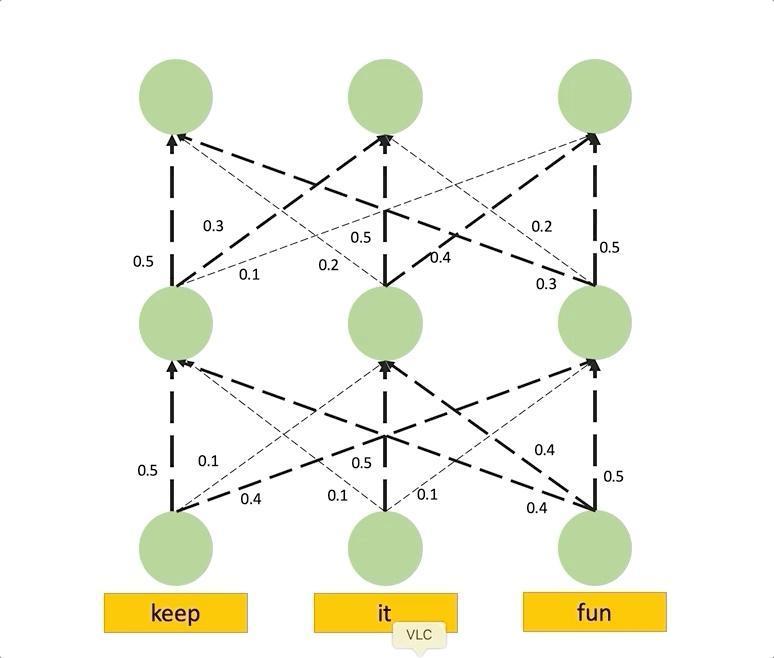
Attention rollout simulation obtained from Samira Abnar’s blog
This is super straight-forward and easy to understand but we are missing the influence of residual connections. Paper authors handle this in a very elegant way, they realize that the output at layer \(V_{l+1}\) depends on the previous output and the attention weights: \(V_{l+1} = V_{l} + W_{att}V_l\), where \(W_{att}\) is the attention matrix. This can also be expressed as \(V_{l+1} = (W_{att} + I)V_l\). Thus, re-normalizing the weights, the raw attention updated by residual connections can be expressed as: \(A = 0.5W_{att} + 0.5I\).
Note I have seen other implementations of this method that instead of averaging the attention between the different heads of each layer, use min or max operator since it seems to work better in practice (see this implementation)
Code
First of all we need to setup our ViT model, unfortunately at the moment of writing this post we cannot use Torchvision’s ViT because it is not included in latest version 0.11.1 (it has been recently added see this PR). For this reason, we cannot use the new feature extractor and we need to find another implementation. I will use Hugging Face library because it is simple and allows me get all attention matrices directly.
from transformers import ViTForImageClassification
vit = ViTForImageClassification.from_pretrained("google/vit-base-patch16-224").to("cuda")
vit.eval()
You can check the official documentation to see how we can use output_attentions parameter to get the attentions tensors of all attention layers. Attention rollout code would consist on:
# Inference
result = vit(img_tensor, output_attentions=True)
# Stack all layers attention
attention_probs = torch.stack(result[1]).squeeze(1)
# Average the attention at each layer over all heads
attention_probs = torch.mean(attention_probs, dim=1)
# Add residual and re-normalize
residual = torch.eye(attention_probs.size(-1)).to("cuda")
attention_probs = 0.5 * attention_probs + 0.5 * residual

# Normalize by layer
attention_probs = attention_probs / attention_probs.sum(dim=-1).unsqueeze(-1)

# Compute rollout
attention_rollout = attention_probs[0]
for i in range(1, attention_probs.size(0)):
    attention_rollout = torch.matmul(attention_probs[i], attention_rollout)

# Attentions between CLS token and patches
mask = attention_rollout[0, 1:]
# Reshape back to 2D
mask_size = np.sqrt(mask.size(0)).astype(int)
mask = mask.reshape(mask_size, mask_size)
Pretty simple, let’s see a few examples:
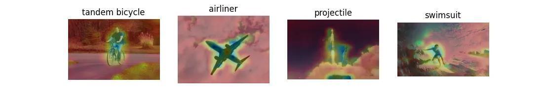
There seems to be a larger noise when we comparing these results wrt CAM ones. One plausible option to reduce this effect is to filter very low attentions and keep only the strongest ones. I will stick with the original implementation but you find about this in this repo.
Conclusion
We have covered two important methods that can give us some intuition on how CNNs and Transformers work internally. A few key aspects that we must keep in mind:
-
The idea behind this post was to improve my understanding of the ViT architecture, TorchVision new features, GAP and Attention Rollout. This should not be used as a comparison between ResNet and ViT, since ViT was pre-trained on ImageNet-21k and finetuned on ImageNet whileas ResNet50 was only trained on ImageNet.
-
CAM does not generalize to models without global average pooling. You would need to retrain your model with a GAP layer or use a different method. Here you can check some different implementations.
-
I have used Hugging Face’s ViT implementation since it is not yet available on latest Torchvision version.
-
Do not forget to check the Hugging Face Space I created for this post!
References
- [1] Zhou, B., Khosla, A., Lapedriza, A., Oliva, A., & Torralba, A. (2016). Learning deep features for discriminative localization. In Proceedings of the IEEE conference on computer vision and pattern recognition (pp. 2921-2929).
- [2] Abnar, S., & Zuidema, W. (2020). Quantifying attention flow in transformers. arXiv preprint arXiv:2005.00928.
- [3] Dosovitskiy, A., Beyer, L., Kolesnikov, A., Weissenborn, D., Zhai, X., Unterthiner, T., … & Houlsby, N. (2020). An image is worth 16x16 words: Transformers for image recognition at scale. arXiv preprint arXiv:2010.11929.
- [4] Khan, S., Naseer, M., Hayat, M., Zamir, S. W., Khan, F. S., & Shah, M. (2021). Transformers in vision: A survey. arXiv preprint arXiv:2101.01169.
Any ideas for future posts or is there something you would like to comment? Please feel free to reach out via Twitter or Github