DVC + MMdetection

I recently published a post where I showed how to use DVC to maintain versions of our datasets so we reduce data reproducibility problems to a minimum. This is the second part of the tutorial where we are going to see how we can combine the power of mmdetection framework and its huge model zoo with DVC for designing ML pipelines, versioning our models and monitor training progress.

It is quite a lot of content to cover, so I will be going through it step by step and trying to keep things as simple as possible. You can find all the code for this tutorial in my Github. So let’s start with it!

1. Setup the environment

We are gonna need a few packages to get our project up and running. I have created a conda.yml that you can find in the root of the repository, this is going to install pytorch and cudatoolkit since we are going to train our models using a GPU. You can create the environment by:

conda env create -f conda.yaml
conda activate mmdetection_dvc

2. Import our dataset

In the previous post we used a subset of the COCO dataset created by fast.ai. We push all data to a Google Drive remote storage using DVC and keep all metada files in a Github repository. We need now to import this dataset in our repo and that’s exactly what dvc import can do for us!

dvc init
dvc import "git@github.com:mmeendez8/coco_sample.git" "data/" -o "data/"

Note that we are importing /data folder of the remote repository into the data/ directory of our project where all our data will be stored. This may take a while since we need to download all images and annotations from the remote gdrive storage. Let’s now publish the changes on git:

git add . 
git commit -m "Import coco_sample dataset" 
git push

Once it is downloaded, we can move between different versions of the dataset with the dvc update command. If we would go back to v1.0 of our dataset and push our changes to git:

dvc update --rev v1.0 data.dvc
git add data.dvc
git commit -m "Get version 1.0 of coco_sample"
git push

That’s it! We have imported our dataset and we know how to move between different versions so let’s create a script that will train our model!

3. Train our model

MMDetection is an open source object detection toolbox based on PyTorch. It is a part of the OpenMMLab project and it is one of the most popular computer vision frameworks. I love it and I am an active contributor since it became my default framework for object detection last year.

They have an extense documentation which really helps first time users. In this post I will skip the very basics and focus on showing how easily can we train a RetinaNet object detector on our coco_sample dataset.

3.1. Model config

First thing we need to do is to find the config file for our model, so let’s explore mmdet model zoo and more specifically RetinaNet section. There’s a bunch of different RetinaNet models there but let’s stick with the base config from the original paper. I have already downloaded this file to my repo and you can find it under configs/retinanet_r50_fpn.py. There are three main sections there:

• The backbone definition, which in our case is a ResNet50. Its weights come from some torchvision checkpoint specified at:

init_cfg=dict(type='Pretrained', checkpoint='torchvision://resnet50'))`

As a curious fact, I checked out official torchvision documentation and it seems this network has been trained with some dataset that is currently lost so there is no chance to reproduce this results…

• The Feature Pyramid Network (FPN) configuration which is useful to find features at different scale levels.

• The classification head and the regression head. They predict labels and bounding boxes regression parameters for each of the anchors of the model. I cannot really go deep how this model works and what anchors are but you should check our repo pyodi if you really want to understand all the details.

3.2 Dataset config

Mmdetection framework also uses config files for datasets. There we define our train and validation data and which types of transformation do we want to apply before images are feed into the network. Since our dataset follows COCO format, I just modified original COCO_detection.py. Note that:

• I removed the test set since we are not going to use one for this tutorial.
• I added a CLASSES variable with our reduced set of labels.

You can check the dataset config file in configs/coco_sample.py

3.3 Train configuration

There are multiple training parameters we can configure using mmdetection. For this simple demo we are going to use the default scheduler (see configs/scheduler.py). It uses SGD and a dynamic learning rate policy and that’s mostly what we need to know for now.

Our runtime definition is under configs/runtime.py and we are going to specify a few interesting things there:

• checkpoint_config: specifies the checkpoint saving frequency
• log_config: allows us to select a specific logger for our training
• custom_hooks: extra hooks that we can insert or create for retrieving or adding functionalities to our training
• workflow: it defines training workflow, this is, how many training epochs do we want to run before a validation one.

Since we are using DVC, we are also going to use the DVCLive hook. DVCLive is an open-source Python library for monitoring the progress of metrics during training of machine learning models. It is a recent and super cool library with git integration and that’s all I need! See how simple is to add this hook:

log_config = dict(
    interval=50,
    hooks=[
        dict(type='TextLoggerHook'),
        dict(type="DvcliveLoggerHook", path="training/metrics"),
    ])

4. Data pipeline

Let’s create our first data pipeline! Ideally (and following DVC docs) we should use dvc run commands so the pipeline gets automatically generated but… I feel more comfortable creating a dvc.yaml and filling it myself.

4.1 Prepare the data

Our COCO annotations are missing a few fields because fast.ai guys considered them unnecessary (they actually are) so they removed all extra fields to reduce the final size of the json. That’s fair enough, but mmdetection needs them so I created a very simple script that will prepare the data for us, you can find it in src/prepare_data.py.

The first step of our data pipeline will prepare our annotation file and save the modified COCO files into prepare_data. You can simply add the following to your dvc.yaml:

stages:
  prepare_data:
    foreach:
      - train
      - val
    do:
      cmd: python src/prepare_data.py
        --coco_file data/coco_sample/annotations/split_${item}.json
        --output_file processed_data/${item}_split_with_ann_id.json
      deps:
        - data/coco_sample/annotations/split_${item}.json
      outs:
        - processed_data/${item}_split_with_ann_id.json

There’s a stage called called prepare_data that run a small for loop over values [train, val] and calls the prepare_data script. See how I have specified the original json files as dependencies and the new one as outputs so DVC knows how to track them.

You can now call run the pipeline with dvc repro and the new annotations file should appear!

4.2 Train the model

I have created a simple training script in src/train.py that adjusts to our needs. You could also use mmdetection train tool since I just applied some minor modifications to it that will allow us to use dvc params.

We can add a new step to our data pipeline that executes our training step. For example this would be enough for running an experiment with our actual configs:

train:
  cmd: python src/train.py
    --dataset configs/coco_sample.py
    --model configs/retinanet_r50_fpn.py
    --schedule configs/schedule_1x.py
    --runtime configs/runtime.py
    --work_dir training/checkpoints
  deps:
    - configs/
    - processed_data
    - src/train.py
  outs:
    - training/checkpoints
  live:
    training/metrics:
      summary: true
      html: true

Note how I have added the live key to notify DVC that our script will be saving metrics in the training/metrics folder. Also, this will generate a html file that we can use to visualize in real time our train progress. So simple!

We can run again DVC repro as many times as we want changing our config files as needed for trying different hyperparameters or model configurations. Nevertheless, DVC guys recommend yo to use DVC experiments when you are tryining different configurations. So that’s what we are going to do! Note this is a recent feature and I had to open a couple issues since I found a couple “bugs” or unexpected behavior such [1], [2].

Let’s do our first training by running dvc exp run! You can monitor training progress by opening your training/metrics.html file:

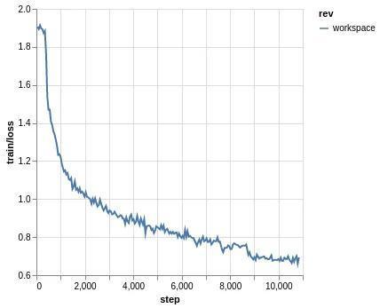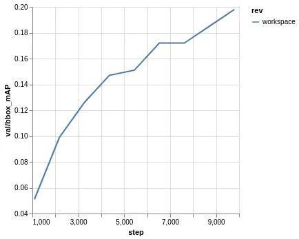Training will be done soon (depening on your GPU and machine) and we can check our results by running:

$ dvc exp show
┏━━━━━━━━━━━━━━━━━━━━━━━━━┳━━━━━━━━━━┳━━━━━━━┳━━━━━━━━━━━━━━━┳━━━━━━━━━━┳━━━━━━━━━━━━━━┳━━━━━━━━━━━━━━━━━┳━━━━━━━━━━━━━━━━━┳━━━━━━━━━━━━━━━━┳━━━━━━━━━━━━━━━━┳━━━━━━━━━
┃ Experiment              ┃ Created  ┃  step ┃ learning_rate ┃ momentum ┃ val.bbox_mAP ┃ val.bbox_mAP_50 ┃ val.bbox_mAP_75 ┃ val.bbox_mAP_s ┃ val.bbox_mAP_m ┃ val.bbox
┡━━━━━━━━━━━━━━━━━━━━━━━━━╇━━━━━━━━━━╇━━━━━━━╇━━━━━━━━━━━━━━━╇━━━━━━━━━━╇━━━━━━━━━━━━━━╇━━━━━━━━━━━━━━━━━╇━━━━━━━━━━━━━━━━━╇━━━━━━━━━━━━━━━━╇━━━━━━━━━━━━━━━━╇━━━━━━━━━
│ workspace               │ -        │ 13057 │         1e-05 │      0.9 │        0.198 │           0.368 │           0.194 │          0.008 │          0.142 │         
│ main                    │ 11:24 AM │     - │             - │        - │            - │               - │               - │              - │              - │         
│ └── cefe59e [exp-acc34] │ 01:20 PM │ 13057 │         1e-05 │      0.9 │        0.198 │           0.368 │           0.194 │          0.008 │          0.142 │         
└─────────────────────────┴──────────┴───────┴───────────────┴──────────┴──────────────┴─────────────────┴─────────────────┴────────────────┴────────────────┴─────────

The possibilty of tracking your hyperparameters is what I most like about experiments. We can change one hyperparameter for a experiment, DVC will remember this for you and will help you to compare different experiments. This is nice but there is room for improvement since at this moment for running an experiment with a different parameter we need to:

1. Add our parameter to our params.yaml
2. Specify that our train step depends on this parameter
3. Run experiment with -S flag updating the parameter value.

These steps are fine when you just change the learning rate or the number of epochs. Nevertheless I consider it does not scales to complex settings where you try a few dozens of different hyperparameters… There is an open issue where I shared my personal opinion, you can go there and read different thinkings since there is a small discussion going on about this new feature.

Let’s increase our L2 regularization or weight decay to see how it affects our results:

# dvc.yaml
train:
  cmd: python src/train.py
    --dataset configs/coco_sample.py
    --model configs/retinanet_r50_fpn.py
    --schedule configs/schedule_1x.py
    --runtime configs/runtime.py
    --work_dir training/checkpoints
  deps:
    - configs/
    - processed_data
    - src/train.py
  outs:
    - training/checkpoints
  live:
    training/metrics:
      summary: true
      html: true
  params:
    - optimizer.weight_decay

# params.yaml
optimizer:
  weight_decay: 0.001 # this is the same value we have in configs/schedule_1x.py

Now we run the experiment with our new value for weight_decay

dvc exp run -S optimizer.weight_decay=0.001

Experiment will start running and once is finished we can compare our results by running:

$ dvc exp show --no-timestamp --include-metrics val.bbox_mAP --include-metrics val.bbox_mAP_50
┏━━━━━━━━━━━━━━━━━━━━━━━━━┳━━━━━━━━━━━━━━┳━━━━━━━━━━━━━━━━━┳━━━━━━━━━━━━━━━━━━━━━━━━┓
┃ Experiment              ┃ val.bbox_mAP ┃ val.bbox_mAP_50 ┃ optimizer.weight_decay ┃
┡━━━━━━━━━━━━━━━━━━━━━━━━━╇━━━━━━━━━━━━━━╇━━━━━━━━━━━━━━━━━╇━━━━━━━━━━━━━━━━━━━━━━━━┩
│ workspace               │          0.2 │           0.371 │ 0.001                  │
│ main                    │            - │               - │ -                      │
│ ├── cefe59e [exp-acc34] │        0.198 │           0.368 │ 0.0001                 │
│ └── 36da522 [exp-6d4ed] │          0.2 │           0.371 │ 0.001                  │
└─────────────────────────┴──────────────┴─────────────────┴────────────────────────┘

Note I have filtered some of the metrics using --include-metrics flag so can easily see the most important ones. It seems that the ‘weight_decay` parameter has an impact on results, and we have been to increase our mAP by 0.01. For this, let’s keep this experiment and commit our changes:

dvc exp apply exp-6d4ed 
git add src/train.py dvc.lock params.yaml dvc.yaml configs processed_data training/metrics.json
git commit -a -m "Save experiment with `weight_decay=.001`"

And finally we can send all our results to respective remotes! These are Github and our Gdrive:

git push
dvc push

We have covered most of the step of the official DVC experiments tutorial. You can go there and check more info about how cleaning up your experiments and how to pull specific ones.

4.3 Results Visualization

We have trained our model and we have an idea of how it performs thanks to the mAP metrics but we all like to the the bounding boxes over our images so we can get a fully understanding of how the model performs! I have create a simple eval script in src/eval.py that will latest model and paint a subset of validation images. We simply need to add a new step to our dvc.yaml:

eval: 
  cmd: python src/eval.py
    --dataset configs/coco_sample.py
    --model configs/retinanet_r50_fpn.py
    --checkpoint_file training/checkpoints/latest.pth
    --output_dir eval/  
    --n_samples 20
    --score_threshold .5
  deps:
    - src/eval.py
    - training/checkpoints/latest.pth
  outs:
    - eval/

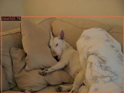
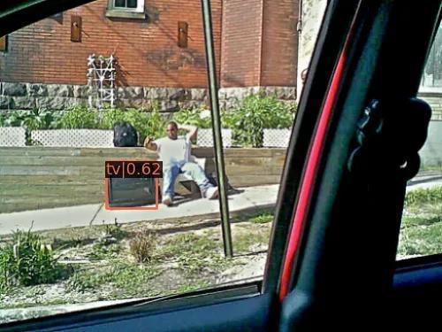
I am going to run dvc repro since I have already commit and pushed my changes from last experiment. This is going to create the eval folder which contains the painted images, see a few examples below:

It seems our model is not perfect… it mistook a fish tank for a TV! Anyway this was expected, the mAP metric is pretty low but even though we can see how it performs pretty well in the other images. You can go and check more results yourself but keep in mind that SOTA models in COCO dataset (80 classes) achieve a mAP ~0.6 and that’s a large difference wrt to our simple model. If you want to know more about COCO ranking I recommend you to check paperswithcode web.

Once we have evaluated our model we can commit and push these results!

git add dvc.lock .gitignore 
git commit -m "Run dvc repro eval"
git push
dvc push

Conclusion

We can use DVC combined with mmdetection to easily train object detection models, compare them and save different versions and experiments. Summarizing this post we have:

• Import a dataset into our repository using dvc import

• Setup a DVC data pipeline and understand how it works

• Train a model using mmdetection:
  • Understand mmdetection config files
  • Take advantage of DVC metrics to configure our trainings and compare experiments
  • Use dvclive to monitor the training progress
• Obtain bbox predictions and paint them over our validation set

Any ideas for future posts or is there something you would like to comment? Please feel free to reach out via Twitter or Github