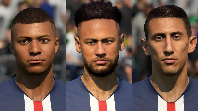
This is my third post dealing with Variational Autoencoders. If you want to catch up with the math I recommend you to check my first post. If you prefer to skip that part and go directly to some simple experiments with VAEs then move to my second post, where I showed how useful these networks can be. If you just want to see how a neural network can create fake faces of football players then you are in the right place! Just keep reading!
I must admit that I would like to dedicate this post…

Note: All code in here can be found on my Github account
You can read the other posts in this series here:
1. Introduction
I spent a few hours thinking about which dataset could I use to apply all the knowledge and lines of code I acquire learning about VAEs.
I had some constraints that limit my work but the main one were the limited availability of resources and computational power. The dataset I was looking for, must had small images which will allow me to get some results in a rational amount of time. Also I would like to deal with colored images, since my previous model was designed for black and white images and I wanted to evolve it to deal with more complex images.
Finally I found a dataset that fitted all my requirements and at the same time was interesting and funny for me, so I could not resist.
2. Data Collection
The dataset I found was upload to Kaggle (more here). It consists on detailed attributes for every player registered in the latest edition of FIFA 19 database. I downloaded the csv file and open a Jupyter notebook to have a look at it.
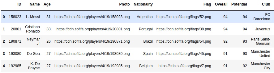
This file contains URLs to the images of each football player. I started by downloading a couple of images to see if links were working well and to check if image sizes were constant. I got good news, links were fine and images seem to be PNG files of 48x48 pixels with 4 different channels (Red, Green, Blue, Alpha).
After this I coded a Python script that could download as fast as possible this dataset. For this I used threads to avoid our CPU to be idle waiting for the IO tasks. You can find the script on Github or implement it by yourself.
I was able to collect a total of 15216 different images since some of the URLs in the csv file were not valid.
3. Data Processing
Yeah! I was able to download our images in a fast way but… when I plotted these images I got the following results:
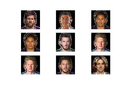
I deduced that someone had applied some preprocessing technique to the edges between the player and the background. So I had to revert this process.
One of the constraints I had in mind was that I had to be able of solving this problem using Tensorflow and nothing else (after all I am trying to improve my skills with it). Alright, so I must implement something that is relatively easy and works like a charm…
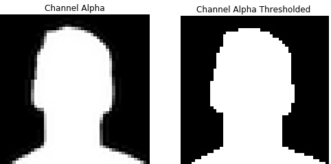
In the Jupyter notebook you can see how I elaborated this method. I basically used the alpha channel (as a boolean mask) and I convert it to a binary image using a certain threshold. After this step I filtered all the pixels in the image that were not present in the mask. This can be easily done in a few lines of code and results are really great! I encourage you to check the notebook since is the easiest way to understand it.
In Tensorflow you can create a simple function that takes a RGBA image as input and returns the reconstructed one (without the alpha channel).
| def remove_noise(image): | |
| alpha = tf.greater(image[:, :, 3], 50) | |
| alpha = tf.expand_dims(tf.cast(alpha, dtype=tf.uint8), 2) | |
| noise_filtered = tf.multiply(alpha, image) | |
| return noise_filtered[..., :3] |
In here I convert the alpha channel into a 48x48 boolean matrix. After this I convert the matrix to uint8 and I add a third dimension to the data so I can apply a wise multiplication with all the channels of the original image. This multiplication will set to zero all those pixels that have a zero value in the mask and I return only the RGB channels. Isn’t it easy?
3. Data Pipe
Now it’s time to create a pipeline for our data. We need to:
-
Read bytes from image files
-
Decode those bytes into tensors
-
Remove noise
-
Convert to tf.float32
-
Shuffle and prefetch data
Tensorflow’s Dataset API allow us to do all these steps in a very simple way.
| def parse_function(filename): | |
| image_string = tf.read_file(filename) | |
| image = tf.image.decode_png(image_string, channels=4) | |
| image = remove_noise(image) | |
| image = tf.image.convert_image_dtype(image, dtype=tf.float32) | |
| image.set_shape([48, 48, 3]) | |
| return image | |
| def load_and_process_data(filenames, batch_size, shuffle=True): | |
| ''' | |
| Reveices a list of filenames and returns preprocessed images as a tensorflow dataset | |
| :param filenames: list of file paths | |
| :param batch_size: mini-batch size | |
| :param shuffle: Boolean | |
| :return: | |
| ''' | |
| with tf.device('/cpu:0'): | |
| dataset = tf.data.Dataset.from_tensor_slices(filenames) | |
| dataset = dataset.map(parse_function, num_parallel_calls=4) | |
| if shuffle: | |
| dataset = dataset.shuffle(5000) # Number of imgs to keep in a buffer to randomly sample | |
| dataset = dataset.batch(batch_size) | |
| dataset = dataset.prefetch(2) | |
| return dataset |
4. Define the network
In my previous post I show how to define the Autoencoder network and its cost function. Nevertheless, I was not happy with that implementation since the definition of the network was in the main file, very far away from what I would consider a modular code.
So now, I have created a new class which will allow me to create the network in a very simple and intuitive manner. I must thank to this amazing post from Danijar Hafner where I found a way to combine decorators with Tensorflow’s Graph intuition. I won’t explain this code in here, otherwise the post would be too long but feel free to ask below about anything you want.
The main advantage of using this decorator is that ensures that all nodes of the model are only created once in our Tensorflow graph (and we save a lot of lines of code).
| import tensorflow as tf | |
| import functools | |
| import numpy as np | |
| def define_scope(function): | |
| # Decorator to lazy loading from https://danijar.com/structuring-your-tensorflow-models/ | |
| attribute = '_cache_' + function.__name__ | |
| @property | |
| @functools.wraps(function) | |
| def decorator(self): | |
| if not hasattr(self, attribute): | |
| setattr(self, attribute, function(self)) | |
| return getattr(self, attribute) | |
| return decorator | |
| class VAE: | |
| def __init__(self, data, latent_dim, learning_rate, image_size=48, channels=3): | |
| self.data = data | |
| self.learning_rate = learning_rate | |
| self.latent_dim = latent_dim | |
| self.inputs_decoder = ((image_size / 4)**2) * channels | |
| self.encode | |
| self.decode | |
| self.optimize | |
| @define_scope | |
| def encode(self): | |
| activation = tf.nn.relu | |
| with tf.variable_scope('Data'): | |
| x = self.data | |
| with tf.variable_scope('Encoder'): | |
| x = tf.layers.conv2d(x, filters=64, kernel_size=4, strides=2, padding='same', activation=activation) | |
| x = tf.layers.conv2d(x, filters=64, kernel_size=4, strides=2, padding='same', activation=activation) | |
| x = tf.layers.conv2d(x, filters=64, kernel_size=4, strides=1, padding='same', activation=activation) | |
| x = tf.layers.conv2d(x, filters=64, kernel_size=4, strides=1, padding='same', activation=activation) | |
| x = tf.layers.flatten(x) | |
| # Local latent variables | |
| self.mean_ = tf.layers.dense(x, units=self.latent_dim, name='mean') | |
| self.std_dev = tf.nn.softplus(tf.layers.dense(x, units=self.latent_dim), name='std_dev') # softplus to force >0 | |
| # Reparametrization trick | |
| epsilon = tf.random_normal(tf.stack([tf.shape(x)[0], self.latent_dim]), name='epsilon') | |
| self.z = self.mean_ + tf.multiply(epsilon, self.std_dev) | |
| latent = tf.identity(self.z, name='latent_output') | |
| return self.z, self.mean_, self.std_dev | |
| @define_scope | |
| def decode(self): | |
| activation = tf.nn.relu | |
| with tf.variable_scope('Decoder'): | |
| x = tf.layers.dense(self.z, units=self.inputs_decoder, activation=activation) | |
| x = tf.layers.dense(x, units=self.inputs_decoder, activation=activation) | |
| recovered_size = int(np.sqrt(self.inputs_decoder/3)) | |
| x = tf.reshape(x, [-1, recovered_size, recovered_size, 3]) | |
| x = tf.layers.conv2d_transpose(x, filters=64, kernel_size=4, strides=1, padding='same', | |
| activation=activation) | |
| x = tf.layers.conv2d_transpose(x, filters=64, kernel_size=4, strides=1, padding='same', | |
| activation=activation) | |
| x = tf.layers.conv2d_transpose(x, filters=64, kernel_size=4, strides=1, padding='same', | |
| activation=activation) | |
| x = tf.layers.conv2d_transpose(x, filters=64, kernel_size=4, strides=1, padding='same', | |
| activation=activation) | |
| x = tf.contrib.layers.flatten(x) | |
| x = tf.layers.dense(x, units=48 * 48 * 3, activation=None) | |
| x = tf.layers.dense(x, units=48 * 48 * 3, activation=tf.nn.sigmoid) | |
| output = tf.reshape(x, shape=[-1, 48, 48, 3]) | |
| output = tf.identity(output, name='decoded_output') | |
| return output | |
| @define_scope | |
| def optimize(self): | |
| with tf.variable_scope('Optimize'): | |
| # Reshape input and output to flat vectors | |
| flat_output = tf.reshape(self.decode, [-1, 48 * 48 * 3]) | |
| flat_input = tf.reshape(self.data, [-1, 48 * 48 * 3]) | |
| with tf.name_scope('loss'): | |
| img_loss = tf.reduce_sum(flat_input * -tf.log(flat_output) + (1 - flat_input) * -tf.log(1 - flat_output), 1) | |
| latent_loss = 0.5 * tf.reduce_sum(tf.square(self.mean_) + tf.square(self.std_dev) - tf.log(tf.square(self.std_dev)) - 1, 1) | |
| loss = tf.reduce_mean(img_loss + latent_loss) | |
| tf.summary.scalar('batch_loss', loss) | |
| optimizer = tf.train.AdamOptimizer(self.learning_rate).minimize(loss) | |
| return optimizer |
5. Put the pieces together
The program will read data from a list of filenames which I locate into a placeholder, since I want to be able to feed it with new data in a near future (after training) to evaluate its performance.
| # Create tf dataset | |
| with tf.name_scope('DataPipe'): | |
| filenames = tf.placeholder_with_default(get_files(FLAGS.data_path), shape=[None], name='filenames_tensor') | |
| dataset = load_and_process_data(filenames, batch_size=FLAGS.batch_size, shuffle=True) | |
| iterator = dataset.make_initializable_iterator() | |
| input_batch = iterator.get_next() | |
| # Create model | |
| vae = VAE(input_batch, FLAGS.latent_dim, FLAGS.learning_rate, ) |
As you can see above, the network class constructor receives the input batch tensor, an iterator that moves through our bank of images. Also, filenames variable corresponds with the previously mentioned placeholder. It has a default value returned by the get_files function which simply lists all filenames that are contained in the directory data_path.
How does this look in TensorBoard? Pretty cool!
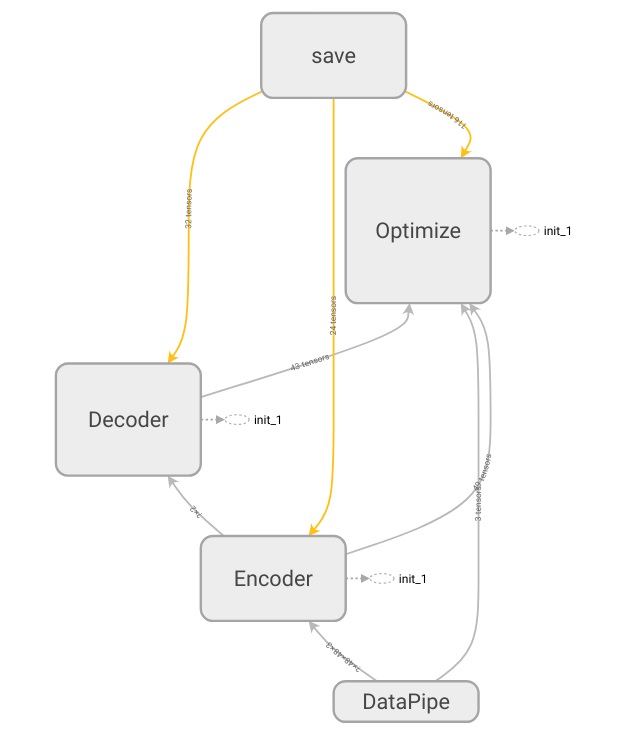
The save block, it’s created to save the network state (weights, biases) and the graph structure (see GitHub for more)
5. Experiments
The training phase is computationally expensive and I am working on my personal laptop so I could not get very far with the number of epochs. I encourage the readers who have more resources to try new experiments with longer workouts and to share their results.
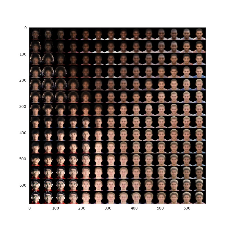
2D Latent Space
One of the coolest things with VAEs, is that if you reduce the latent space to just two dimensions, you will be able to deal with data in a 2 dimensional space. So you move your data from a 48x48x3 dimensional space to just 2! This allows you to get visual insights about how is the model distributing the data around the space. I did this for a total of 500 epochs and I force the net to return both input images and the reconstructed ones, in order to see, if the network was able to reconstruct the original inputs.
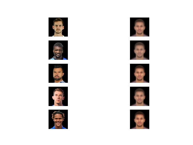
Reconstruction at epochs 2, 150 and 500 (top to bottom)
As we can see, at epoch 2, the reconstructed images are almost all the same. It seems the networks learns the pattern of a ‘general’ face and it simply modifies its skin color. At epoch 150 we can see greater differences, the reconstruction is better but still far from reality, though we start to see different hair styles. At epoch 500, the reconstruction did not succeed, but it learn to differentiate the most general aspects of each face and also some expressions.
Why are these results so poor compared with our previous work with MNIST datasets? Well, our model is too simple. We are not able to encode all the information in a 2 dimensional space, so a lot of it is being lost.
But we still can have a look to our 2 dimensional grid space and force the network to create some fake players for us! Let’s have a look below:
This is what we got! Interesting result… but we already knew this was going to happen isn’t it?. The network is too simple, so this ‘standard faces’ that we see are made of similar football players profiles. This means that our encoder is doing a good job, placing similar faces in close regions in the space BUT the decoder is not able to reconstruct a 48x48x3 image from just 2 points (which is, in fact, a super hard task). This is why the decoder is always outputting similar countenances.
What could we do? Well, we can increase the complexity of our model and add some extra dimensions to our latent space!
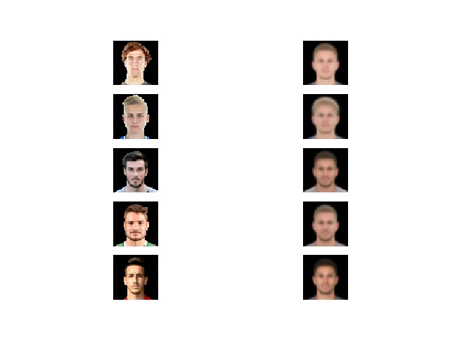
15D Latent Space
Let’s repeat the training with a total 15 dimensions in our latent space and check how our face reconstructions are evolving with the training. For this I have trained the network during 1000 epochs.
I discovered Floydhub a Deep Learning platform that allows me to use their GPUs for free (during 2 hours). This fact, allowed me to perform this long training phase. I really recommend to try Floydhub, since it is really easy to deploy your code and run your training there.
Update: FloydHub was shutdown at 5:00pm Pacific Time on Friday, August 20, 2021.
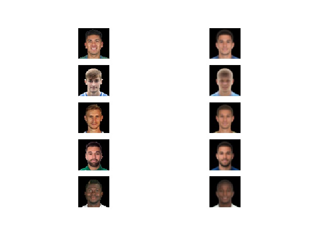
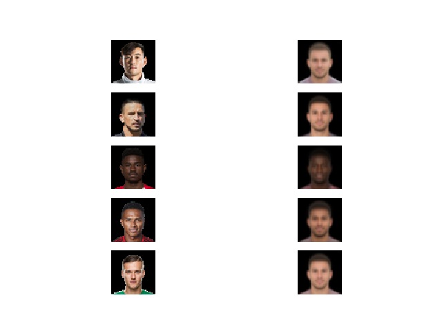
Reconstruction at epochs 150 and 1000
It seems our network is doing a better job now! The reconstructions have improved and they really look like the original input. Let’s note the jersey colors, the haircuts and the face positions! But is this good enough? Can you guess the original input from these reconstructions?
Well, it’s pretty hard to imagine the original input for these reconstructed faces… From left to right these are Messi, Ronaldo, Neymar, De Gea and De Bruyne. A longer training or another complexity increasement would produce better results so I encourage you to get my code on Github and give it a try!
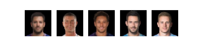
Interpolate points
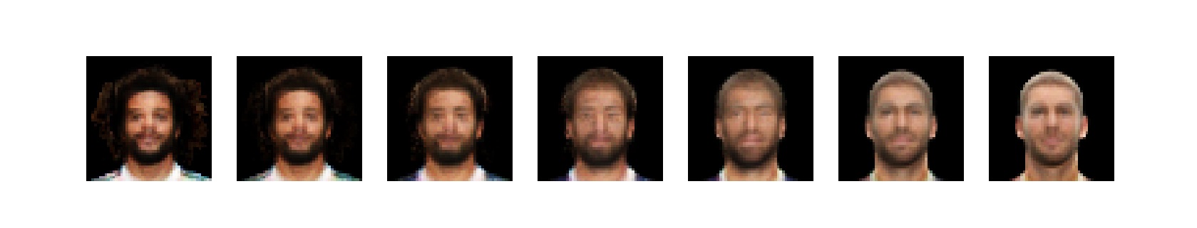
We know that our encoder will place each image in a specific point of our 15 dimensional space. So if get two images we will have two different points in that latent space. We can apply a linear interpolation between them, in order to extract other points.
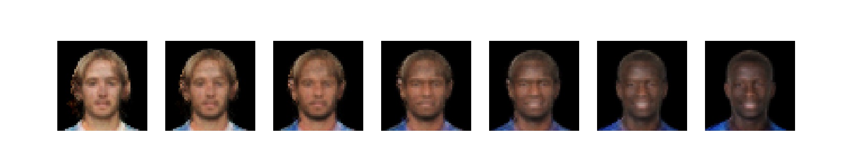
This is the result when we get Modric and Kante’s latent vector and we interpolate a total of 5 points between them. We can observe how moving around our latent space make us obtain different facial features. You can try as many combinations as you want!
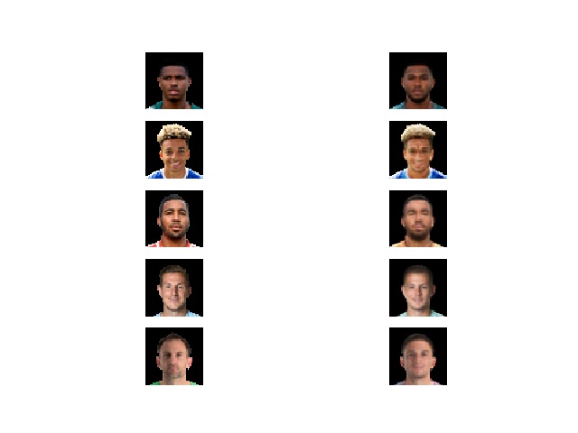
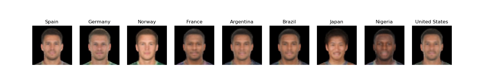
Average player by country
If you are used to work with machine learning, you have heard about unsupervised learning and the importance of centroids on this field. A centroid can be defined as the mean point of all those that belong to the same cluster or set.
Our data is categorized by skills, football team, age, nationality… So imagine the following, we could get all the players for a certain country, let’s say Spain, and obtain the latent vector that our encoder produces for each one of them. After this we can compute an average of these latent vector and encode it, in a way, that we are obtaining an image of a fake player that has the most common facial features for a certain country!! How cool sounds that?
You can observe the most common attributes for each country collected in a single image.
Conclusion
In this post we have learnt how to apply VAEs to a real dataset of colored images. I have shown how to preprocess the data and how to create our network in a structured way. The experiments I have collected are just a reduced set of the huge amount of possibilities that one can obtain after dealing with image embeddings (our latent space vectors).
I would like to encourage you to try the code, create new experiments, use different dimensional spaces or longer trainings!
Any ideas for future posts or is there something you would like to comment? Please feel free to reach out via Twitter or Github