In my previous post I covered the theory behind Variational Autoencoders. It’s time now to get our hands dirty and develop some code that can lead us to a better comprehension of this technique. I decided to use Tensorflow since I want to improve my skills with it and adapt to the last changes that are being pushed towards the 2.0 version. Let’s code!
Note: All code in here can be found on my Github account
Get the data
Tensorflow (with the recently incorporated Keras API) provides a reasonable amount of image datasets that we can use to test the performance of our network. It is super simple to import them without loosing time on data preprocessing.
Let’s start with the classics and import the MNIST dataset. For this, I will use another recently added API, the tf.dataset, which allows you to build complex input pipelines from simple, reusable pieces.
In here we download the dataset using Keras. After this we create tensors that will be filled with the Numpy vectors of the training set. The map function will convert the image from uint8 to floats. The dataset API allows us to define a batch size and to prefetch this batches, it uses a thread and an internal buffer to prefetch elements from the input dataset ahead of the time they are requested. Last three lines are used to create an iterator, so we can move through the different batches of our data and reshape them. Pretty simple!
If this is the first time you use this API I recommend you to test how is this working with this simple example that shows the first image of each batch.
Easy isn’t it? Alright, let’s keep moving.
Encoder
We must now “code our encoder”. Since we are dealing with images, we are going to use some convolutional layers which will help us to maintain the spatial relations between pixels. I got the some of the ideas of how to structure the network from this great Felix Mohr’s post
My intention is to gradually reduce the dimensionality of our input. The images are 28x28 pixels, so if we add a convolutional layer with a stride of 2 and some extra padding too, we can reduce the image dimension to the half (review some CNN theory here). With two of these layers concatenated the final dimensions will be 7x7 (x64 if have into account the number of filters I am applying). After this I use another convolutional layer with stride 1 and ‘same’ padding which will maintain the vector size through the conv operations.
The mean and standard deviation of our Gaussian will be computed through two dense layers. We must note that the standard deviation of a Normal distribution is always positive, so I added a softplus function that will take care of this restriction (other works also apply a diagonal constraint on these weights). The epsilon value will be sampled from an unit normal distribution and then we will obtain our \(z\) value using the reparametrization trick (see my previous post)
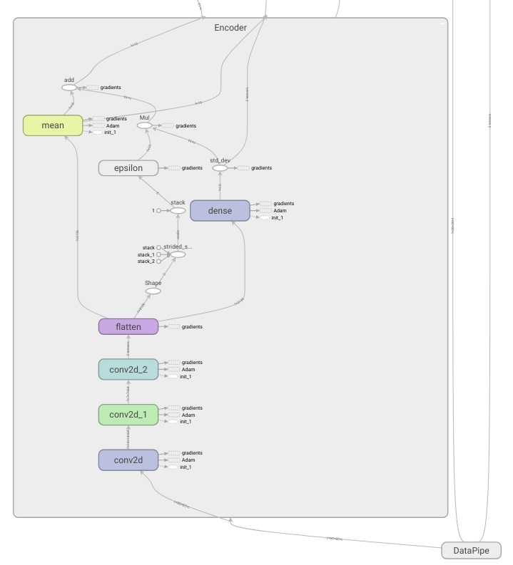
Tip: we can see how our network looks using TensorBoard! (full code on Github)
Decoder
When we speak about decoding images and neural networks, we must have a word in our mind, transpose convolutions! They work as an upsampling method with learning parameters, so they will be in charge of recovering the original image dimension from the latent variables one. It’s common to apply some non linear transformations using dense layers before the transposed ones. Below we can observe how the decoder is defined.
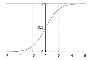
Note that FLAGS.inputs_decoder references the number of neurons in our dense layers which will determine the size of the image before the transpose convolution layers. In this case I will use the same structure as in the encoder, so the number of neurons will be 49 and the input image size to the first tranposed conv layer will be 7x7. It’s also interesting to point that the last layer uses a sigmoid activation, so we force our outputs to be between 0 and 1.
Cost function
We have defined out encoder and decoder network but we still need to go trough a final step which consists on joining them and defining the cost function that will be optimized during the training phase.
I first connected the two networks and then (for simplicity sake) I have reshaped input and output batches of images to a flat vector. After this the image loss is computed using the binary cross entropy formula, which can be interpreted as the minus log likelihood of our data (more in here). We move on and compute the latent loss using the KL divergence formula (for a Gaussian and a unit Gaussian) and finally, we get the mean of all the image losses.
That’s all! We have created a complete network with its corresponding data input pipeline with just a few lines of code. We can move now, test our network and check if it can properly learn and create new amazing images!
Experiments
1. Are our networks learning?
Let’s start with a simple example and check that the network is working as it should. For this we will use the MNIST and fashion MNIST datasets and see how is the network reconstructing our input images after a few epochs. For this I will set the number of latent dimensions equal to 5.
Below, we can see how our network learns to transform the input image in the latent space of 5 dimensions, to recover them then to the original space. Note how as more epochs have passed, we obtain better results and a better loss.
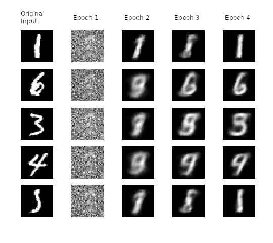
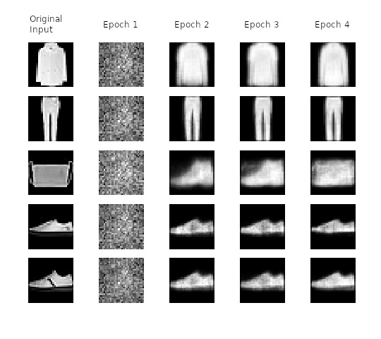
Image recovering vs epoch number for MNIST and Fashion MNIST datasets
We see how our network keeps improving the quality of the recovered images. It’s interesting to see how at the initial epochs numbers 6, 3, 4 are converted into something that we can considered as “similar” to a 9. But, after a few iterations the original input shape is conserved. For the fashion dataset we get a similar behavior with the bag pictures that are initially recovered as a boot!
It’s also curious, to observe how the images change to get an intuition of what is happening during the learning. But what is going on with the image encodings?
2. How does our latent space look?
In the previous section we used a 5 dimensional latent space but we can reduce this number to a two dimensional space which we can plot. In this way the complete images will be encoded in a 2D vector. Using a scatter plot, we can see how this dimensional space evolves with the number of epochs.
In a first moment all images are close to the prior (all point are located around 0). But during training the encoder learns to approximate the posterior distribution, so it will locate the latent variables in different parts of the space having into account their labels (equal label -> close region in the space). Let’s have a look first and then discuss more about this!
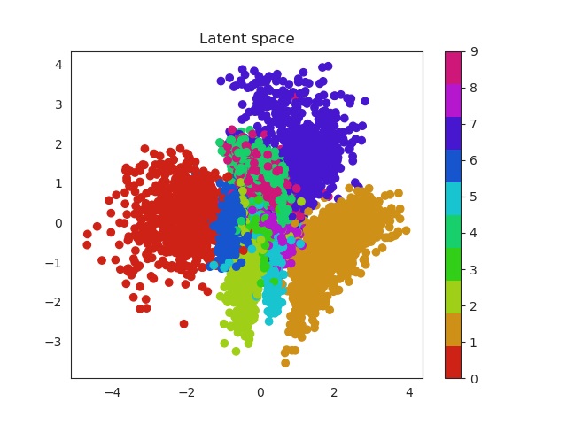
MNIST latent space evolution during 20 epochs
Isn’t this cool? Numbers that are similar are placed in a similar region of the space. For example we can see that zeros (red) and ones (orange) are easily recognized and located in a specific region of the space. Nevertheless it seems the network can’t do the same thing with eights (purple) and threes (green). Both of them occupy a very similar region.
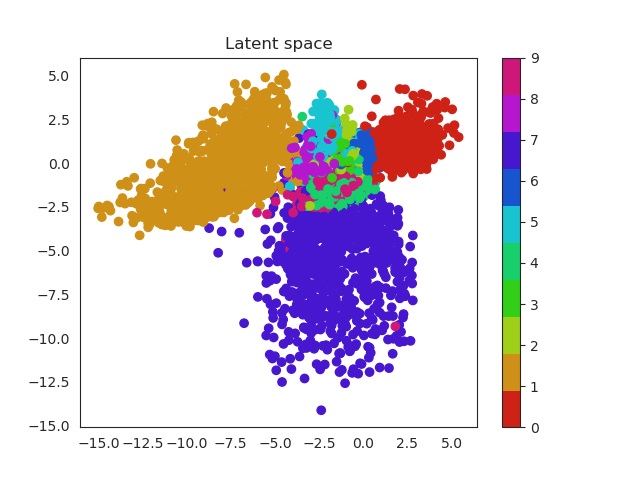
Same thing happens with clothes. Similar garments as shirts, t-shirt and even dresses (which can be seen as an intersection between shirts and trousers) will be located in similar regions and the same thing happens with boots, sneakers and sandals!
Fashion MNIST latent space evolution during 20 epochs
These two dimensional plots can also help us to understand the KL divergence term. In my previous post I explained where does it come from and also that acts as a penalization (or regularization term) over the encoder when this one outputs probabilities that are not following an unit norm. Without this term the encoder can use the whole space and place equal labels in very different regions. Imagine for example two images of a number 1. Instead of being close one to each other in the space, the encoder could place them far away. This would result in a problem to generate unseen samples, since the space will be large and it will have ‘holes’ of information, empty areas that do not correspond to any number and are related with noise.
Latent space without KL reg
Latent space with KL reg
Look the x and y axis. On the left plot, there is not regularization, so points embrace a much larger region of the space, while as in the right image they are more concentrated, so this produces a dense space.
3. Generating samples
We can generate random samples that belong to our latent space. These points have not been used during training (they would correspond with a white space in previous plots). Our network decoder though, has learnt to reconstruct valid images that are related with those points without seem them. So let’s create a grid of points as the following one:
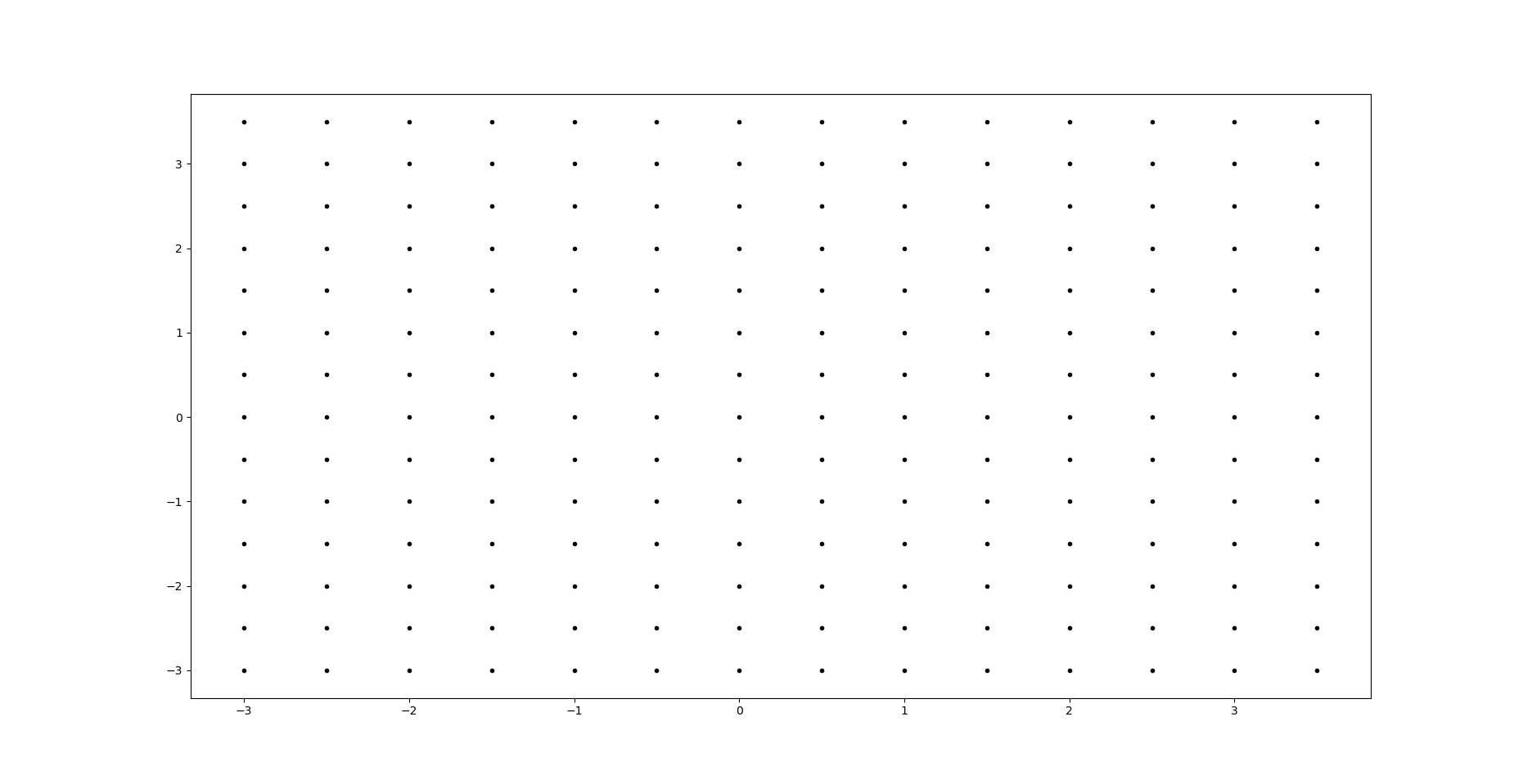
Each of this points can be passed to the decoder which will return us a valid images. With a few lines we can check how is our encoder doing through the training and evaluate the quality of the results. Ideally, all labels would be represented in our grid.
Comparsion between grid space generated images and latent space distribution
What about the fashion dataset? Results are even more fun! Look how the different garment are positioned by ‘similarity’ in the space. Also the grid generated images look super real!

After 50 epochs of training and using the grid technique and the fashion MNIST dataset we achieve these results:
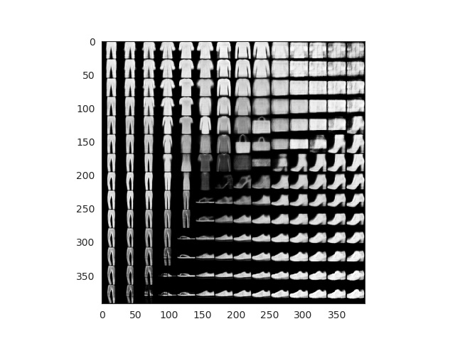
Fake images generated using mesh grid points
All this images here are fake. We can finally see how our encoder works and how our latent space has been able to properly encode 2D image representations. Observe how you can start with a sandal and interpolate points until you get a sneaker or even a boot!
Conclusion
We have learnt about Variational Autoencoders. We started with the theory and main assumptions that lie behind them and finally we implement this network using Google’s Tensorflow.
-
We have used the dataset API, reading and transforming the data to train our model using an iterator.
-
We have also implemented our encoder and decoder networks in a few lines of code.
-
The cost function, made up of two different parts, the log likelihood and the KL divergence term (which acts as a regularization term), should be also clear now.
-
The experimental section was designed to support all the facts mentioned above so we could see with real images what is going on under all the computations.
It could be interesting to adapt our network to work with larger and colored images (3 channels) and observe how our network does with a dataset like that. I might implement some of these features but this is all for now!
Any ideas for future posts or is there something you would like to comment? Please feel free to reach out via Twitter or Github