The theory behind Variational Autoencoders

Generative models are one of the cooler branches of Deep Learning. During last weeks Generative Adversarial Networks (GANs) have been present in a large number of posts (most of them related with Nvidia’s last work). Thanks to this I realized that, although I had studied generative models at University, I had never code even one of them! So I decide to change this panorama and spend a couple hours (re)learning about Variational Autoencoders. In these series of post I will try to transmit and also to provide useful resources which I have found and I feel in the need of transmit!

What are VAEs?

Variational Autoencoders are after all a neural network. They consist of two main pieces, an encoder and a decoder. The first of them is a neural network which task is to convert an input datapoint \(x\) to a hidden or latent representation \(z\), with the characteristic that this encoding has a lower number of dimensions than the original output. So, the encoder works as a compressor, that ‘summarizes’ the data into a lower dimensional space.

The decoder is also neural network. It’s input will be in the same dimensional space than the encoder’s output and its function consists on bringing the data back to the original probability distribution. This is, output an image as the ones we have in our dataset.

So during training, the encoder ‘encodes’ the images into the latent space (information is lost due to lower dimensionality), after this the decoder tries to recover the original input. The commited error is for sure backpropagated through the whole network and the this improves its ability to reconstruct the original inputs.

But wait… wasn’t this a generative model? Yes! The encoder is in fact fitting a probability distribution to our data! The lower dimensional space is stochastic (usually modeled with a Gaussian probability density), so once our training has converged to an stable solution, we can sample from this distribution an create new unseen samples!!

If you are not impressed yet, think about this simplification of the problem. Imagine we collect all articles that have been published in New York Times during last year and we force ourselves to summarize them but with the following restriction: we can only use one hundred words from English vocabulary. For this task we will need to select this set of words carefully to minimize the loss of information. When we have succeed at this task, we might be able to reconstruct the original article from the words we see. But also, we can select a random number of words (from the 100 sample set) and create a new ‘fake’ article!

We will then act as encoders, transforming the articles into a reduced 100 words space. The decoder task will be based on recovering as much as possible of the original article!

The math

My idea here is to stick just with those parts that were more difficult to understand for me and that might help another person in the same situation! I will cover the intuition behind the algorithm and the most important parts that one needs to understand before implementing this network on on Tensorflow.

There are two main resources I have used where you can find a whole explanation of VAEs algorithm. These are Doersch article and Jaan Altosaar blog post.

The variational autoencoder can be represented as a graphical model. Where the joint probability can be expressed as \(p(x, z) = p(x\|z) p(z)\). So latent variables (the lower representation) and data points can be sampled from \(p(z)\) and \(p(x\|z)\) respectively.

Graphical model representation obtained from Jaan’s blog

What we in fact want, is to find good values for the latent variables given our dataset, which is known as the posterior \(p(z\|x)\). We can use Bayes rule to calculate this value by: \(p(z\|x) = p(x\|z)p(z) / p(x)\). Nevertheless \(p(x)\) cannot be efficiently computed since it has to be evaluated over all possible \(z\) (\(z\) can be any distribution!!). So here is where things get interesting. VAEs assume that samples of \(z\) can drawn from a simple distribution. We can then approximate the posterior using only a family of distributions. But why does this strong approximation can work? Well, in own Doersch words:

“The key is to notice that any distribution in d dimensions can be generated by taking a set of d variables that are normally distributed and mapping them through a sufficiently complicated function”

Which I would express in another way as: do not worry, it is a simplification but the neural network will take care of it!

The family of distributions can be expressed as \(q​_λ​​(z∣x)\). The \(λ\) term refers to a specific family, if we are working with Gaussians, then \(λ\) will Zcorrespond with the mean and variance of the latent variables for each datapoint.

So we use \(q(z\|x)\) to approximate \(p(z\|x)\). We can use Kullback-Leibler divergence to measure how well are we approximating p.

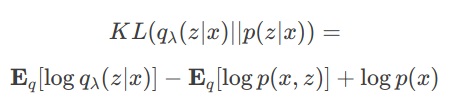
We need to minimize this divergence but, once again, we find the intractable term \(\log p(x)\). Nevertheless we can rewrite this into an intuitive way. Let’s define the Evidence Lower BOund function (ELBO) as:

This functions is a lower bound on the evidence, this means that if we maximize it, we will increase the probability of observing the data (more here). If we mix the two previous equations we will get:

And it is known that KL divergence is always greater or equal than zero. So… maximizing the ELBO is all we need to do and we can get rid of the KL divergence term.

In our neural network the encoder takes input data and outputs \(λ\) parameters that approximate \(q​_θ​​(z\|x, λ)\) and the decoder gets latent variables into the original data distribution \(p_ϕ(x\|z)\). This \(θ\), \(ϕ\) are the neural networks weights. So we can write the ELBO function (unwrapping the joint probability term) as:

This is our lost function! We must highlight two things from here. First of all, we can apply backpropagation to this function (the previous equation is defined for single datapoints). Second, a lost function in Deep Learning is always minimized, so we will have to work with the negative ELBO.

That’s all! Although it might seem a little convoluted at the beginning, I have found the ELBO trick super interesting! You must think that we have found a tractable solution from an intractable problem by reducing our hypothesis set (our family of distributions will be Gaussian) and applying a small amount of math!

Gaussian tricks!

As we said before, the family of distribution that we are going to use are Gaussians. Usually, \(p(Z) = Normal(0,1)\), so if the encoder outputs representations of \(z\) which are not following a unit normal distribution, will get penalized by the KL divergence term (more info on KL divergence between Gaussians here)

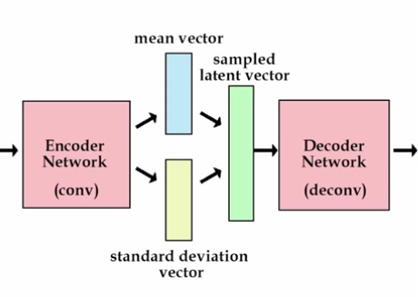
Decoder will sample z from \(q​_θ​​(z\|x)\). The problem here is that backprop will not be able to flow through this random node since it is purely stochastic and non deterministic on networks parameters. We can enforce this, knowing that a normal distributed variable with mean \(μ\) and standard deviation \(σ\), can be sampled from:

where \(ϵ\) is drawn from a standard normal. Why is this helping us? Think that now we are dealing with fixed values for \(μ\) and \(σ\), we are moving all the stochasticity to the epsilon term so the derivatives can flow through the deterministic nodes! (Note that in image below \(ϕ\) corresponds with our \(θ\) term)

*

Image obtained from Kingma’s talk

In this video you can find a good visual explanation of the whole network!

---

Conclusion and next steps

In this post I have covered the basic intuition we must have in order to implement a Deep Variational Autoencoder. In next posts we will go through the implementation of this network using tensorflow, we will evaluate some of the obtained results playing with different dimensions of our latent space and observe how our data distributes on it. I must once again thank to the amazing article written by Doersch who has helped me to properly understand the theory behind VAEs.

Any ideas for future posts or is there something you would like to comment? Please feel free to reach out via Twitter or Github